Optimizing the pipeline: Data
Chapter 4 of the Training at Larger Scale series
Optimizing the pipeline: Data
Efficient data loading can significantly reduce training time and costs
- The GPU (or TPU/HPU etc.) is the most expensive and performance-critical component in a training pipeline.
- If the data pipeline (i.e., loading, preprocessing, transferring) is slow, the GPU will sit idle, waiting for the next batch.
What You Want
- A data pipeline that saturates the GPU as much as possible without introducing too much memory pressure or over demanding CPUs.
- Each DataLoader worker is effectively a producer that loads data in parallel, while your training loop (running on the main process/GPU) is the consumer. The goal is to maximize overlap: while one batch is being processed on the GPU, the next batch (or several batches) are being loaded by the CPU workers in the background.
4. Optimizing the pipeline: Data/
├── benchmark_datapipeline_configurations.py  # Main benchmark script
├── plot_benchmark_runs.ipynb                # Analysis notebook
├── dummydataset.py                          # Dummy dataset for testing
├── utils.py                                 # Utility functions
├── benchmark_logs/                          # Benchmark results
└── benchmark_imgs/                          # Visualizations
Key Concepts and Metrics
-
GPU Saturation: The key performance target.
-
CPU (cores):
- Used by the main process and workers to (lazy) load, transform, and prepare data for training. You want high CPU usage (busy workers) but not so high that the OS or other processes starve. If your CPU utilization is peaking at 100% on all cores and the system becomes unresponsive or the throughput plateaus, you may have too many workers or threads.
- You can check available CPUs using:
import os print(os.cpu_count()) -
RAM (used by CPU processed tasks):
- Used by workers to load batches into memory.
- Important when working with large datasets, large batch sizes, or complex transforms.
vRAM (used by GPU):
- During model training weights, gradients and calculations are stored here.
-
I/O Considerations
-
Bandwidth: The maximum rate of data transfers (e.g., from cloud storage to your instance)
-
Chunking: Use optimal chunk sizes to balance I/O overhead and memory usage
-
File Formats: Choose ML-optimized formats (Parquet, TFRecord, WebDataset, Zarr)
-
-
Streaming Workers (Dask) vs DataLoader Workers (PyTorch)
PyTorch DataLoader and streaming frameworks like Dask can be combined effectively to stream cloud data into your training pipeline, but it’s crucial to understand they operate at different layers of the data process:
-
PyTorch DataLoader manages the training-specific data handling by:
- Creating worker processes to parallelize sample preparation
- Implementing batching, shuffling, and sampling strategies
- Executing the preprocessing defined in your
__getitem__method - Transferring prepared batches to the GPU
-
Streaming frameworks (e.g. Dask) handles the low-level data access by:
- Building a computational graph (DAG) for lazy loading
- Managing how data chunks are read from storage
- Orchestrating parallel fetching of data from cloud/disk
These systems don’t automatically coordinate with each other. The connection point occurs when a DataLoader worker calls
__getitem__on your Dataset, which then triggers Streaming frameworks (e.g. Dask) to materialize the required data chunks when calling a.load()function. By understanding this separation, you can optimize each layer independently:- Configure optimal data reading (e.g. chunk sizes, thread count, worker count)
- Configure DataLoader for optimal batch preparation (e.g. num_workers, prefetch_factor)
It’s important to avoid conflicting parallelism between these systems because too many concurrent processes and threads can lead to resource contention and degraded performance.
-
Benchmarking: Practical guidelines and background
I have created scripts to help you optimize your data pipeline, but before we dive into the benchmarking and optimization, it is important to understand how everything works.
Understanding DataLoader Workers and Process Distribution When optimizing your data pipeline, it’s important to understand how worker processes are distributed across your available CPU cores and to leave sufficient CPU resources for main processes and system overhead. Reserve 1-2 CPU cores per GPU for the main training process and system overhead. When using containerization solutions like Docker, you may need to reserve additional CPU resources for container management.
-
Single GPU setup: With a single GPU and one main training process, you’ll have a single DataLoader that spawns
num_workersprocesses. For example, on a machine with 20 CPU cores and 1 GPU, you should reserve 1-2 cores for the main process and system overhead, leaving about 18 cores for DataLoader workers. -
Multi-GPU setup: With multiple GPUs (e.g., using DistributedDataParallel), each GPU has its own main process, and each main process creates its own set of DataLoader workers. For instance, on a machine with 8 GPUs and 160 CPU cores, you should reserve 8-16 cores for main processes and system overhead (1-2 per GPU), leaving approximately 144-152 cores to be distributed among all worker processes.
To avoid CPU contention, ensure the total number of worker processes does not exceed your available cores minus those needed for the main process. Without torch.compile, the main thread orchestrating the GPU (especially for high-performance hardware like an H100) can become a bottleneck if it has to compete with data workers. To prevent this, set num_workers = total_cores - 1 to keep one core dedicated to GPU control. While slight oversubscription can be beneficial when workers are idling on I/O, prioritizing a free core for the main process is generally safer unless torch.compile is used to reduce CPU overhead.
Batch size The set batch size is important as it dictates how much data is loaded into memory at once. The ideal batch size depends on your dataset characteristics, model complexity, and available GPU memory. You want a batch size that enables stochastic gradient descent, while having a stable enough learning signal. For my use case, 32 worked well, but you may need to adjust this based on your specific requirements. This batch size is needed because it is used in my optimization benchmark script later.
Cloud vs. Local Performance: Note that network bandwidth varies dramatically between environments. When moving from local (WiFi) to cloud training, you may see orders of magnitude improvement in data loading speed. In my case, I observed a 100x decrease in wait time when moving to the cloud. Always benchmark in the same environment where you’ll be training, as the optimal configuration can differ significantly between local and cloud setups. High bandwidth allows more data to flow per second, while low bandwidth creates bottlenecks that can leave your GPU waiting for data.
No need to over-optimize the DataLoader: If your model is small or the GPU is not very powerful, there’s no point in using 16+ workers or heavy parallel jobs when the GPU is already saturated. I have spent quite some time doing research on this, and it is important to think about this step as it can drastically increase your performance, but there is no need to do “grid search” such-like stuff for this. Follow my guide and your speed should already improve a lot. Experimenting endlessly with this also costs money and potential experimentation time. I’ll tell you more on how to do it in a sec.
What can be optimized: dataset
Dataset-level optimization is about making data access as efficient as possible. By storing data smartly (chunked, compressed appropriately, possibly colocated with training if remote), and by only doing the minimal necessary work for each access, you ensure that the raw data supply is fast. Once that is in place, DataLoader-level tuning can further amplify the throughput. If there are no parameters, chunking or file format to be optimized, focus on the dataloader instead. (when streaming from machine’s disk memory, ssd or when streaming is all handled automatically). If applicable to your usecase, I will show how to approach this in the Appendix.
What can be optimized: dataloader
The DataLoader is critical for training performance. Key parameters to optimize:
-
num_workers: Controls parallel data loading subprocesses- Too few: GPU waits for data
- Too many: Resource contention, diminishing returns
- NOTE: num_workers is not about CPU’s but processes, and a process may use more or less than 1 cpu core.
-
prefetch_factor: Batches loaded in advance per worker- Default is 2, which works for most cases
- Adjust based on sample size and memory requirements
- Total prefetched =
num_workers * prefetch_factor
-
pin_memory: Enables faster CPU to GPU transfers- Set to
Truewhen using GPU - Creates page-locked memory for direct transfers
- Slightly increases CPU memory usage
- Set to
-
persistent_workers: Keeps workers alive between epochs- Reduces worker initialization overhead
- Useful for large datasets and complex initialization
- Significantly reduces epoch transition time
-
multiprocessing_context: Controls worker process spawning- Options: ‘fork’, ‘spawn’, ‘forkserver’
- Use ‘forkserver’ (or ‘spawn’) for better CUDA compatibility
- Note: for more detail, you can read the Pytorch docs
Even with an efficient dataset, proper DataLoader settings are crucial.
Optimizing: Benchmarking Tools for DataLoader Optimization
I created two files to help you optimize your data pipeline:
-
- suitable for any pytorch Dataset object
- Runs and logs different DataLoader configurations
- Measures performance metrics for each configuration
- Includes Dask integration (commented out by default for those who don’t need it)
- Contains a configurable
train_step_timeparameter (default: 0.1 seconds)- This simulates model training time
- You can set this to match your actual model’s training time per batch
- The goal remains the same: minimize data loading wait times
-
- Jupyter notebook for visualizing benchmark results
- Creates charts comparing different configurations
- Helps identify the optimal setup for your specific hardware
How to optimize with the benchmark scripts
Follow these steps to systematically optimize your data pipeline:
- Import your own dataset by changing the line on top of
benchmark_configurations.py.
from dummydataset import DummyDataset as YourDataset # replace with your dataset
-
Optional: Measuring the time it takes to (load a mini batch and) complete a single training step. This information is useful for properly configuring the benchmark script parameters to accurately reflect your real-world training conditions. For this, you can run the
timing_benchmark.pyscript that is in the folder of 4. Optimizing the pipeline: Model. and then change thetrain_step_timeparameter in thebenchmark_configurations.pyscript. -
Establish a baseline Start with minimal configuration:
-
num_workers = 0(single-process loading) -
prefetch_factor = None(default behavior) persistent_workers = Falsepin_memory = False
-
-
Implement a sensible default configuration
- E.g. for a system with 10 CPU cores and 1 GPU:
- Reserve 1-2 cores for the main training process
- Allocate remaining cores between DataLoader workers (and streaming processes)
- Example allocation:
- 3 cores for Dask streaming workers (if using Dask)
- 5 cores for DataLoader workers
- E.g. for a system with 10 CPU cores and 1 GPU:
-
Experiment with different configurations
- Test variations systematically:
- More streaming workers, fewer DataLoader workers
- More DataLoader workers, fewer streaming workers
- Higher CPU oversubscription
- Optional: Even higher oversubscription
- Lower CPU oversubscription
- Different
prefetch_factorvalues
- Test variations systematically:
-
Run benchmarks and analyze results
- Use
benchmark_configurations.pyto test all configurations - Can be run locally or in the cloud
- (Download and) analyze the files with
plot_benchmark_runs.ipynb(use the*.logfiles, not the*_workers.logfiles. They make sure the*.logfiles are correct) - Compare performance metrics across configurations
- Use
Use the plotting notebook to visualize differences between runs and identify which configuration has the lowest wait/batch fetching time. I do not explicitly measure vRAM/CPU utilization in these tools, the primary goal is to significantly improve training time with reasonable effort. Having that said, watch for these warning signs:
- Memory issues: If memory usage spikes, reduce workers, prefetch factor, or caching.
- Diminishing returns: If adding workers doesn’t improve throughput, you’ve reached saturation.
Example Benchmark Results
Below are example benchmark results showing the significant difference between an unoptimized baseline configuration and an optimized one:

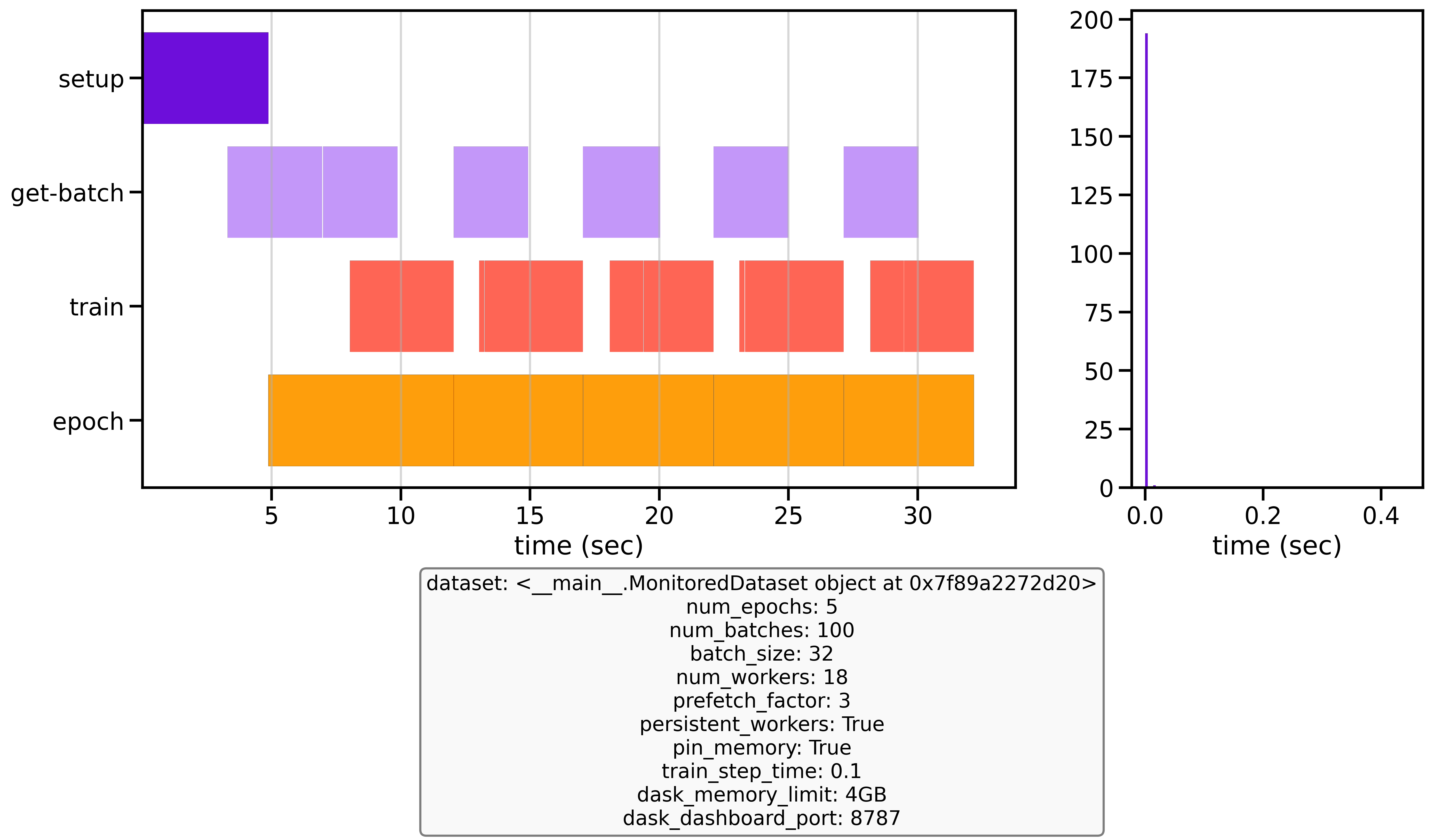
Unoptimized baseline vs optimized configuration performance after 3 epochs with 50 batches
With these simple optimizations, my dataloader became 35 times faster than the baseline. Earthmover, who made the first version of this benchmark script was able to run 15x faster. This performance improvement is transformative for training - where others might only complete 4 epochs in a given timeframe, I was able to run 140. This acceleration dramatically reduces overall training time, costs and allows for more experimentation and model iterations.
Now that we have the data-part of the pipeline optimized, lets focus on optimizing the Model