Appendix
Chapter 7 of the Training at Larger Scale series
Appendix
Here you can find the additional information as referenced in the chapters.
1. Overview of advantages of Lightning over Raw PyTorch
| Feature | PyTorch | Lightning |
|---|---|---|
| Device/GPU Handling | Manual device placement (.to(device)), manual multi-GPU management | accelerator="auto", devices="auto" handles single GPU, multi-GPU (DDP), TPU, CPU fallback |
| Training Loop | Manual train/eval mode, gradient zeroing, loss, backward, optimizer steps | Handled in training_step, validation_step |
| Logging | Manual print or custom logging | Built-in TensorBoard, WandB, MLflow, auto metric aggregation, progress bars |
| Callbacks | Manual implementation | Built-in model checkpointing, early stopping, learning rate monitoring |
| Multi-GPU Strategies | Manual data parallelism, distributed training, gradient synchronization | Specify strategy parameter in Trainer |
| Profiling & Debugging | Manual profiling setup | Built-in profilers and debugging tools |
| Reproducibility | Manual seed setting everywhere | seed_everything() (Note: manual seed for data loader/workers still needed) |
| Mixed Precision Training | Manual AMP implementation | precision="16-mixed" in Trainer |
| Automatic Sanity Checks | No built-in pre-training validation | Sanity validation batch (model forward pass, shape compatibility, loss calculation). Disable with num_sanity_val_steps=0. |
| Cloud Storage Integration | Manual cloud storage uploads | Easy integration via custom callbacks for checkpoint uploads (e.g., AWS S3, GCS). Prevents data loss, customizable backup strategies. |
2. Optimizing the Dataset
-
Efficient Storage Formats:
Initially, my data was stored in NetCDF files, which are common for scientific data but can be inefficient when working with streaming from cloud storage. The default chunking in these files was not optimized for machine learning, causing unnecessary data to be loaded into memory during training. To address this, I stored everything in Zarr. Zarr is specifically designed for fast cloud-based data access. I will not include the migration in this blog, as it is out of scope, I just want to show that it is important to think about the data formats used.
Zarr v3 Performance Tip
When using Zarr v3, you can achieve a significant speedup by disabling Dask during dataset loading. By setting
chunks=None, you bypass Dask’s graph-building overhead and allow Xarray to use its internal lazy-indexing. This is often faster because Zarr v3’s own storage layer is already optimized for concurrent I/O.# Optimal Zarr v3 loading dataset = xr.open_zarr( path, consolidated=False, zarr_format=3, chunks=None ) -
Optimal Chunking:
When streaming data, the goal is to minimize both the amount of data loaded and the number of individual chunk requests made.
- Too small chunks: Results in many small I/O requests, creating overhead
- Too large chunks: Loads unnecessary data, wasting bandwidth and memory
I created a script to (handwavy) calculate the optimal chunk size by analyzing how different chunk dimensions affect data access patterns. For an image of 64x64 pixels:
chunk_size minimal_chunks maximal_chunks minimal_bytes maximal_bytes 8x8 64 81 4096 5184 16x16 16 25 4096 6400 32x32 4 9 4096 9216 64x64 1 4 4096 16384 128x128 1 4 16384 65536 256x256 1 4 65536 262144 512x512 1 4 262144 1048576 1024x1024 1 4 1048576 4194304 The table shows how different chunk sizes affect loading efficiency:
- Minimal chunks: Fewest number of chunks needed to load the image data
- Maximal chunks: Worst-case number of chunks needed (when image spans multiple chunks)
- Minimal/maximal bytes: Corresponding data volume that must be transferred
The results show that a 64×64 chunk size (matching the image dimensions) provides the optimal balance:
- It requires loading only 1-4 chunks per image
- The data volume ranges from 4,096 to 16,384 bytes
- Larger chunk sizes (128×128+) dramatically increase the bytes loaded
- Smaller chunk sizes (8×8 to 32×32) require substantially more chunk requests
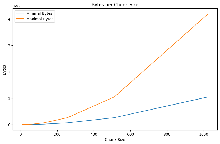
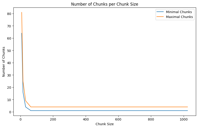
Number of bytes and chunks for different chunk sizes
Handling the Small File Bottleneck
Optimizing Zarr chunks can inadvertently create millions of small files (inodes) On servers with poor small-file I/O, this can cripple training speed even if your chunk sizes are technically “optimal.” A powerful solution is SquashFS, which packs your entire dataset into a single compressed, read-only filesystem image. By mounting this image, your code sees the original directory structure, but the hardware only manages one large file, drastically reducing overhead. This combination of SquashFS and Zarr v3 is particularly effective for static datasets on high-performance clusters where metadata lookups are the primary bottleneck. This is out of scope for this blog, but do reach out if you need help!
-
Parallelize I/O: Loading Efficiently
Some libraries, like Dask, can parallelize reading within a dataset, providing their own optimization parameters. However, be careful when combining these with PyTorch DataLoader workers, as this can lead to resource contention and diminishing returns.
When working with lazy-loading/streaming data into GPU memory, there are several parameters you might need to optimize:
-
Parallel Loading Parameters:
- Number of concurrent readers/workers (processes that execute computations)
- Memory limits per worker (to prevent OOM errors)
- Thread pool size per worker (for parallel execution within a worker)
-
Caching Parameters:
- Cache size limits (to prevent OOM errors)
- Cache eviction policies (to prevent OOM errors)
- Persistent vs. in-memory caching (to prevent OOM errors)
I will explain how to optimize these (usecase) parameters in the next section. For more insights on optimizing cloud data loading, see Earthmover’s guide to cloud-native dataloaders covering streaming techniques, I/O optimization, and resource balancing. Note that this is relevant for zarr v2. In zarr v3, as mentioned above, we disable dask and set chunks=none for an even bigger speedup.
-
3. Optimizing Dask
If you’re using Dask, you can also leverage the Dask dashboard to monitor:
- Worker memory usage
- CPU utilization
- Task execution
- Resource bottlenecks
Understanding Dask Execution Modes
Dask offers three execution modes, each with different trade-offs:
-
Single-Threaded Scheduler
- Uses
dask.config.set(scheduler="single-threaded") - All tasks run sequentially in the main thread
- No parallelism but minimal overhead
- Useful for debugging or when relying entirely on DataLoader’s parallelism
- In multi-GPU setups, each process runs its own sequential scheduler
- Uses
-
Threaded Scheduler
- Uses
dask.config.set(scheduler="threads", num_workers=dask_threads) - Tasks run in parallel using a thread pool within a single process
- Good for I/O-bound operations (like reading data chunks)
- Moderate parallelism with low overhead
- In multi-GPU setups, be careful of the total thread count (e.g., 8 processes × 4 threads = 32 threads)
- Uses
-
Distributed Cluster
- Uses
LocalClusterandClientto create a full Dask cluster - Runs multiple worker processes, each with multiple threads
- Provides process-level parallelism, bypassing Python’s GIL
- Includes a dashboard for monitoring tasks and resource usage
- Options for per-GPU-process clusters or a single shared cluster
- Higher overhead but better isolation and monitoring capabilities
For a single GPU with limited CPUs (e.g., 20 cores):
- A threaded scheduler with 4-8 threads is often sufficient
- A small distributed cluster (1-2 workers, 4 threads each) offers better monitoring
For multi-GPU setups (e.g., 8 GPUs with 20 cores):
- Be careful not to oversubscribe your CPU resources
- If each GPU process uses its own Dask cluster, limit to 1 worker with 2 threads per process
- Consider using a single shared Dask cluster for all GPU processes
- Monitor CPU utilization to avoid contention
The key is balancing parallelism against resource constraints. More parallelism isn’t always better, especially when resources are shared across multiple GPU processes. Start conservative and scale up while monitoring performance.
- Uses
-
Caching and Locality: For remote data, implement caching strategies to avoid repeatedly downloading the same data.
4. Profiling: Check Your Pipeline
What is it?
Profiling helps you understand where time and resources are spent in your training pipeline. It guides optimization by identifying bottlenecks. The profiler also looks at the data part of the pipeline, so it is a good idea to run it after the data part is done.
How does it work?
Look at the provided script to profile your training loop. Import your dataloader and model modules, then run the script 3 times with the three profilers:
- Simple Profiler
- Advanced Profiler
- PyTorch Profiler (Chrome Trace Viewer)
it stores the output in the output/profiler/{config_name}/profiler_logs folder.
uv run python profiler.py
Interpreting Profiler Outputs – A Quick Guide
Understanding what the profiler outputs mean is key to optimizing your training pipeline. Here’s what to look for in each profiler and how to make sense of the data.
1. fit-simple_profiler_output.txt – Summary View (Simple Profiler)
What it shows:
- High-level summary of function calls
- Average time per operation
- Relative contribution of each function to total runtime
How to read it:
- Look at the top-consuming operations — these are usually bottlenecks.
- Pay attention to data loading functions (
*_dataloader_next,__next__) — these often take more time than expected. - Training loops like
run_training_epochwill typically be a large portion; the key is to ensure they’re not dwarfed by overheads.
When to take action (example):
- If data loading takes a large share of total time (e.g., >40%), your pipeline is I/O-bound.
- If your model training steps are taking less time than preprocessing, you’re likely under-utilizing the GPU.
2. fit-advanced_profiler_output.txt – Line-Level View
What it shows:
- Function-level granularity (per-call stats)
- Total calls, total time, average time per call
- Stack trace to locate the exact code path
How to read it:
- Sort by total time and identify high-call-count, low-time ops — these may be optimized or batched.
- Use stack traces to pinpoint performance sinks inside your own code or framework code.
- Investigate setup or utility functions being called excessively (e.g., synthetic data generation, logging, checkpointing).
When to take action (example):
- If any function is causing a lot of time, (where you expect it to be fast) check if it is necessary.
3. pt.trace.json – Chrome Trace Viewer (PyTorch Profiler)
What it shows:
- Frame-by-frame execution timeline
- Operator-level breakdown (CPU and GPU)
- Optional memory usage tracking
How to read it:
- Open Chrome and go to
chrome://tracing. - Drop in the
.jsonfile. - Hover over timeline blocks to see operator names, start/end times, and device usage.
What to look for:
- Long horizontal bars → slow operations (usually backward passes, large convolutions)
- Gaps between ops → potential I/O waits or CPU/GPU syncs
- Overlapping CPU/GPU ops → good utilization
- Memory heatmaps (if enabled) → identify peaks or leaks
When to Take Action (example):
- If any function is causing a lot of time, (where you expect it to be fast) check if it is necessary.
- If idle gaps exist, investigate DataLoader efficiency